Optimal Design of Discrete Choice Experiments with DB-error
A key step in designing an efficient Discrete Choice Experiment (DCE) is to select the best set of groups of alternatives to show to the participants. I understand here the best set of groups of cards as the set of grouped alternatives to display to the participants that brings the most information to the researcher, i.e., that allows us to estimate as precisely as possible the parameters of the latent utility function that we seek to estimate.
In what follows, I show how to use the DB-error method and design an R algorithm to select the best set of alternatives. This post is inspired by the paper that introduces the R package idefix (link) and this blog post from DisplayR (link). The objective is to show how to create an algorithm the select the best set of grouped cards « by hand ».
Theoretical framework
Let us consider the following general framework that relies on the Multinomial Logit Model (MNL) developed by McFadden (1984). Imagine that we ask an individual i to select one alternative in a group of alternatives (that we call the choice set s). For each alternative k in the choice set s, the participant derives a utility that is made of a systematic (i.e., certain) part noted \(V_{ik}\) and that we assume to be equal to:
\( V_{ik} = X_{ik} \beta \)
where \(X_{ik}\) is the matrix of characteristics of alternative k and/or individual i.
The stochastic utility further contains an error term \(\epsilon_{ik}\) and can be written as follows:
\(U_{ik}=V_{ik}+\epsilon_{ik}\)
where \(\epsilon_{ik}\) is assumed to be identically and independently distributed according to a Gumbel distribution.
The probability for individual i to choose alternative k in the choice set s is given by:
\(p_{iks}(\beta)=\frac{exp(X_{ik} \beta)}{\sum_{l\in s} exp(X_{il} \beta)}\)
where \(l \in s\) represents all the alternatives displayed in the choice set s. Note that this model assumes the Independence of Irrelevant Alternatives (IIA) which states that the utility that one derives from alternative k does not depend on the characteristics of other alternatives. (But the probability to choose alternative k depends of course on the characteristics of the other alternatives.)
Note that the above equation is used in Maximum Likelihood Estimation (MLE) to estimate the parameters \(\beta\).
D-error
Remember that in MLE, the standard errors of the estimates are estimated using the inverse of the Fisher Information Matrix (FIM). The D-error score reflects the size of the standard errors of our estimates, by computing the (r-th root of the) determinant of the variance-covariance matrix of our estimates (where r is the number of parameters to estimate). So, our objective is to minimize the D-error score such as to minimize the standard errors of our estimates, i.e., to have the most precise estimates possible. From a practical point of view, we first compute the expected FIM (\(I_{FIM}\)) and then compute the D-error score.
The expected FIM is given by the opposite of the expected hessian matrix of the likelihood function, which is equal to:
\(I_{FIM}(\beta | X)=N \sum_{s=1}^{S} X_s^T (P_s – p_s p_s^T) X_s \)
where \(p_s\) is the vector of probabilities for the choice set s (i.e., the first element corresponds to the probability to choose alternative 1, etc.), \(P_s\) is the diagonal matrix that contains in the diagonal the probabilities of each alternative (\(p_{s1}, p_{s2}, …, p_{sK} \)) (here the choice set s contains K alternatives), and N is the number of participants facing the choice set s in the experiment.
The D-error that we seek to minimize is given by:
\(\text{D-error}=\text{det}(\Omega)^{1/r} \text{ with } \Omega=I_{IFM}(\beta|X)^{-1}\)
where r is the number of parameters to estimate.
DB-error
To compute the actual D-error score of an experiment, we would need to know the parameters \(\beta\). However, we are computing the D-error score in the first place because we do not know the values of \(\beta\) and we try to estimate them. So, we can at best approximate the D-error score by assuming some values for \(\beta\). However, if our guess is incorrect, we might end up with a suboptimal design. To limit the impact of an incorrect assumption on the true values of \(\beta\), we can instead assume a distribution of beliefs (priors) about the true value of the parameters we seek to estimate. For instance, instead of assuming \(\beta_1=2\), we can assume \(\beta_1 \sim N(2,1)\). In other words, we may not be able to say that \(\beta_1\) is equal to 2 for sure, but we can say that \(\beta_1\) is close to 2 (our prior belief corresponds to a normal distribution centered at 2).
Let us note \(\pi(\beta)\) the prior distribution. We can compute the average D-error, we which call the DB-error (B stands for Bayesian), as follows:
\(\text{DB-error} = \int \text{det}(\Omega)^{1/r} \pi(\beta) d\beta\)
We can see that the DB-error score is the weighted average of the D-error score for all possible values of \(\beta\) considered in our priors.
To put it in a nutshell, our objective is to minimize the DB-error score as it should lead to low standard errors for our estimates. Several techniques have been proposed to find the optimal sets of choices that minimize the DB-error score, see for instance the paper that introduces idefix (link). I focus below on the approach taken by Oppe et al. (2022, link) that uses (a large number of) random draws.
Example
Let us consider a case where we want to elicit people’s preferences for plant-based burgers that might vary in three attributes: (i) the price, (ii) the sauce (none – default, ketchup, or mustard), and (iii) the topping (none, onions, or tomatoes).
The fixed part of the latent utility is given by:
\(V_i=\beta_0+\beta_1 price_i + \beta_{21} K_i + \beta_{22} M_i + \beta_{31} O_i + \beta_{32} T_i \)
where K, M, O, and T are dummy variables equal to 1 if there is ketchup, mustard, onions, or tomatoes respectively, or 0 otherwise.
Note that, often, we are interested in the price premium people are willing to pay for the sauce or the topping. In this case, we are interested in estimating \(\beta_i/\beta_1\).
We consider an experimental design where participants must choose one out of two displayed burger alternatives. Imagine that alternatives 1 and 2 are displayed to the participant. We consider here the Multinomial Logit Model presented above and assume that the probability to choose alternatives 1 and 2 is given by:
\(p_1=\frac{exp(V_1)}{exp(V_1)+exp(V_2)}\), \(p_2=1-p1\)
Practical example – Computing the D-error for a given experiment
First, let us start by computing the D-error for a given experiment. Imagine for instance that some colleagues come to you with a given design, and you want to evaluate the D-error score of their design. Your colleagues proposed the following choice sets:
Choice set #1: 6$ – No sauce – Tomatoes OR 6.5$ – Ketchup – Tomatoes
Choice set #2: 7$ – No sauce – Tomatoes OR 6.5$ – Mustard – Tomatoes
Choice set #3: 7$ – No sauce – Onions OR 7.5$ – Mustard – Onions
Choice set #4: 7.5$ – Ketchup – Onions OR 7.5$ – Mustard – Onions
Choice set #5: 6.5$ – No sauce – Onions OR 7.5$ – No sauce – Ketchup
Your colleagues further tell you that 30 participants will face each choice set. They tell you that they anticipate a price premium of $0.75 for the Ketchup, $1 for the Mustard, $1.25 for the onion topping, and $1.5 for the tomatoes. They believe that the baseline utility of eating the burger without any sauce or topping is about $6.
First, let us create the experimental design table in R:
#Generate experimental table
designTable=rbind(c(1,1,1,6,0,0,0,1),
c(1,2,1,6.5,1,0,0,1),
c(2,1,1,7,0,0,0,1),
c(2,2,1,6.5,0,1,0,1),
c(3,1,1,7,0,0,1,0),
c(3,2,1,7.5,0,1,1,0),
c(4,1,1,7.5,1,0,1,0),
c(4,2,1,7.5,0,1,1,0),
c(5,1,1,6.5,0,0,0,0),
c(5,2,1,7.5,1,0,0,0))
designTable=data.frame(designTable)
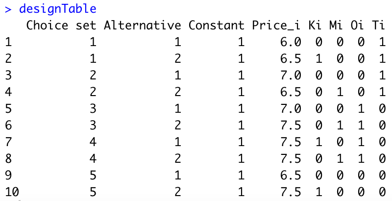
colnames(designTable)=c("Choice set","Alternative","Constant","Price_i","Ki","Mi","Oi","Ti")We obtain the following:
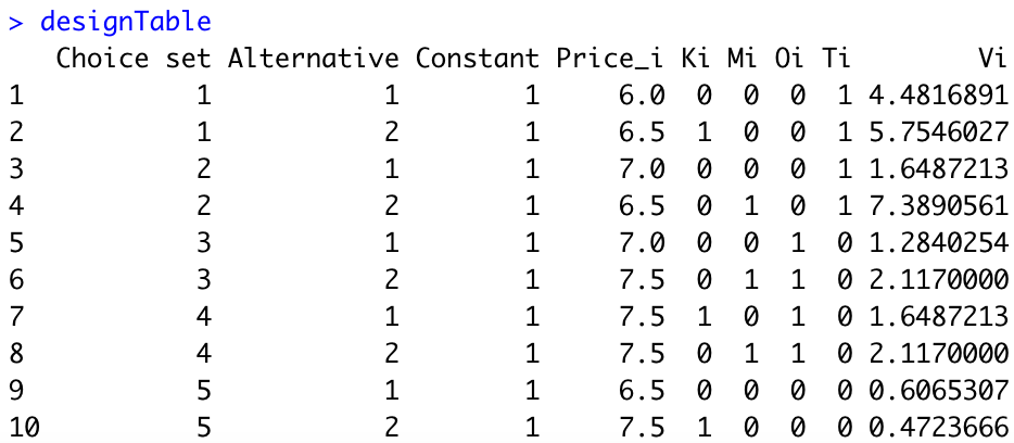
Second, we need to compute the utilities \(V_{ik}\) for each alternative. We assume that \(\beta_1=-1\) (i.e., when the price increases by 1 dollar, the utility decreases by 1 point). The assumptions of your colleague imply that \(\beta_{21}=0.75\), \(\beta_{22}=1\), \(\beta_{31}=1.25\), and \(\beta_{32}=1.5\). Here is the R code:
#Set parameters
beta_0=6
beta_1=-1
beta_21=0.75
beta_22=1
beta_31=1.25
beta_32=1.5
beta=c(beta_0, beta_1, beta_21, beta_22, beta_31, beta_32)

#Generate utilities
designTable$Vi=exp(as.matrix(designTable[,3:8])%*%beta)
We obtain the following:
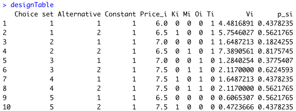
Third, we need to compute the probabilities \(p_{si}\) for each alternative of each choice set. Here is the R code:
#Generate probabilities
designTable$p_si=NA
for(s in 1:5){
  designTable[2*s-1,]$p_si=designTable[2*s-1,"Vi"]/(designTable[2*s-1,"Vi"]+designTable[2*s,"Vi"])
  designTable[2*s,]$p_si=1-designTable[2*s-1,]$p_si
}
We obtain the following:
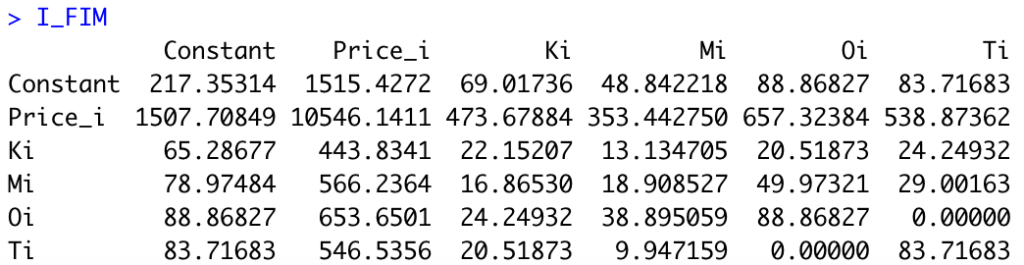
Next, we can compute the Fisher Information Matrix in R:
#Compute Fisher Info Matrix
N=30 #Number of participants
I_FIM=matrix(data=0, nrow=6, ncol=6)
for(s in 1:5){
  X_s=as.matrix(designTable[(2*s-1):(2*s),3:8])
  p_is=diag(designTable[(2*s-1):(2*s),"p_si"])
  P_s=diag(p_is)
  I_FIM=I_FIM+N*t(X_s)%*%(P_s-p_is%*%p_is)%*%X_s
}
I_FIM
We obtain the following matrix:
Last, we need to compute the r-th root of the determinant of the inverse of the FIM. In R:
#Compute the D-error:
Derror=det(solve(I_FIM))^(1/length(beta))
Derror
The D-error for the design and the priors of your colleagues is equal to 0.441.
Practical example – Computing the DB-error for a given experiment
We now turn to the DB-error. Your colleagues are not fully certain of their assumptions about the values of \(\beta\). They believe that the true values of \(\beta\) should be not too far from the value that they provided you. So, you compute the DB-error by assuming a normal distribution with the mean equal to the value that they provided you but with a standard deviation of 0.1.
We first start by creating a function that returns the D-error for any belief vector:
#We create a function that returns the D-error for a given vector beta-funct
returnDerror=function(beta_funct){
  designTable_funct=designTable[,1:8]
  designTable_funct$Vi=exp(as.matrix(designTable_funct[,3:8])%*%beta_funct)
  designTable_funct$p_si=NA
  for(s in 1:5){
    designTable_funct[2*s-1,]$p_si=designTable_funct[2*s-1,"Vi"]/(designTable_funct[2*s-1,"Vi"]+designTable_funct[2*s,"Vi"])
    designTable_funct[2*s,]$p_si=1-designTable_funct[2*s-1,]$p_si
  }
  I_FIM_funct=matrix(data=0, nrow=6, ncol=6)
  for(s in 1:5){
    X_s=as.matrix(designTable_funct[(2*s-1):(2*s),3:8])
    p_is=diag(designTable_funct[(2*s-1):(2*s),"p_si"])
    P_s=diag(p_is)
    I_FIM_funct=I_FIM_funct+N*t(X_s)%*%(P_s-p_is%*%p_is)%*%X_s
  }
  return(det(solve(I_FIM_funct))^(1/length(beta_funct)))
}
We then randomly draw values for the vector of beta’s and we compute the average D-error, which is the DB-error. The R code is as follows. (Note that we set the seed to replicate the results.)
library(mvtnorm)
set.seed(123)
D=1000
vecDerrors=rep(NA,D)
beta_drawn=rmvnorm(D,mean=beta,sigma=diag(rep(0.1,length(beta))))
for(d in 1:D) vecDerrors[d]=returnDerror(beta_drawn[d,])
DBerror=mean(vecDerrors)
The DB-error given the priors and D=1000 random draws is equal to 0.04452939.
Practical example – Optimizing the experiment
We start by creating the list of all possible pairs:
#Generate all unique pairs
allCards=expand.grid(price = c(5.5,6,6.5,7,7.5,8,8.5), ketchup = 0:1, mustard=0:1, onion=0:1, tomato=0:1)
allCards=allCards[!(allCards$ketchup==1 & allCards$mustard==1),] #Remove with both sauces
allCards=allCards[!(allCards$onion==1 & allCards$tomato==1),] #Remove with both toppings
allPairs=expand.grid(card1=1:dim(allCards)[1],card2=1:dim(allCards)[1])
allUniquePairs=allPairs[allPairs$card1>allPairs$card2,] #Get unique pairs

#Generate function to randomly select list of pairs
library(dplyr)
generateListPairs=function(numberOfPairs_funct){
  return(sample_n(allUniquePairs, numberOfPairs_funct))
}
We modify a bit the function that computes the D-error. In some cases, we might not be able to estimate all the parameters (for instance, the design is such that a parameter is never varies). The function would then return an error (i.e., the Fisher Matrix will not be invertible). We take this into account by catching the error.
#We create a function that returns the D-error for a given vector beta-funct
returnDerror=function(beta_funct){
  designTable_funct=designTable[,1:8]
  designTable_funct$Vi=exp(as.matrix(designTable_funct[,3:8])%*%beta_funct)
  designTable_funct$p_si=NA
  for(s in 1:5){
    designTable_funct[2*s-1,]$p_si=designTable_funct[2*s-1,"Vi"]/(designTable_funct[2*s-1,"Vi"]+designTable_funct[2*s,"Vi"])
    designTable_funct[2*s,]$p_si=1-designTable_funct[2*s-1,]$p_si
  }
  I_FIM_funct=matrix(data=0, nrow=6, ncol=6)
  for(s in 1:5){
    X_s=as.matrix(designTable_funct[(2*s-1):(2*s),3:8])
    p_is=diag(designTable_funct[(2*s-1):(2*s),"p_si"])
    P_s=diag(p_is)
    I_FIM_funct=I_FIM_funct+N*t(X_s)%*%(P_s-p_is%*%p_is)%*%X_s
  }
  resDerror=tryCatch({
      return(det(solve(I_FIM_funct))^(1/length(beta_funct)))
    }, error=function(err){
      return(NA)
    })
  return(resDerror)
}
We then generate a function to return the DB-error:
#Generate function to return DB-error
returnDBerror=function(D_funct){
  vecDerrors_funct=rep(NA,D_funct)
  beta_drawn_funct=rmvnorm(D_funct,mean=beta,sigma=diag(rep(0.1,length(beta))))
  for(d in 1:D_funct) vecDerrors_funct[d]=returnDerror(beta_drawn_funct[d,])
  return(mean(vecDerrors_funct, na.rm=TRUE))
}
Last, we generate a loop to randomly select lists of pairs (M=1000 random designs). I use the simulated values beta to ensure that all designs are evaluated under the same conditions. I use here parallel processing to increase the speed of the algorithm.
#Generate loop
library(doParallel)
set.seed(1234)
M=1000
vecDBerror_loopM=rep(NA,M)
cores=detectCores() #Number of
cores
cl <- makeCluster(cores[1]-1, setup_timeout = 0.5)
registerDoParallel(cl)
for(m in 1:M){
print(m)
listPairs_loop=generateListPairs(5)
designTable=matrix(data=NA,ncol=8,nrow=10)
designTable[1,]=as.matrix(cbind(1,1,1,allCards[listPairs_loop[1,1],]))
designTable[2,]=as.matrix(cbind(1,2,1,allCards[listPairs_loop[1,2],]))
designTable[3,]=as.matrix(cbind(2,1,1,allCards[listPairs_loop[2,1],]))
designTable[4,]=as.matrix(cbind(2,2,1,allCards[listPairs_loop[2,2],]))
designTable[5,]=as.matrix(cbind(3,1,1,allCards[listPairs_loop[3,1],]))
designTable[6,]=as.matrix(cbind(3,2,1,allCards[listPairs_loop[3,2],]))
designTable[7,]=as.matrix(cbind(4,1,1,allCards[listPairs_loop[4,1],]))
designTable[8,]=as.matrix(cbind(4,2,1,allCards[listPairs_loop[4,2],]))
designTable[9,]=as.matrix(cbind(5,1,1,allCards[listPairs_loop[5,1],]))
designTable[10,]=as.matrix(cbind(5,2,1,allCards[listPairs_loop[5,2],]))
designTable=data.frame(designTable)
colnames(designTable)=c("Choice set", "Alternative", "Constant", "Price_i", "Ki", "Mi", "Oi", "Ti")
#Returns DB-error
vecRes=foreach(i=1:D, .combine='cbind') %dopar% {
returnDerror(beta_drawn[i,])
}
res_m=mean(vecRes, na.rm=TRUE)
#Save the optimal design so far
if(m==1) optimalDesign=designTable
if(m>1 & !is.na(res_m)) if(res_m<min(vecDBerror_loopM, na.rm = TRUE)) optimalDesign=designTable
#Save results
vecDBerror_loopM[m]=res_m
}
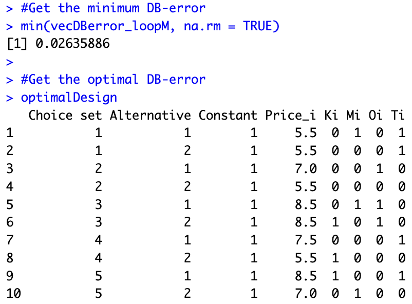
stopCluster(cl)The results of the estimation show that, given our beliefs, we can substantially improve the experimental design compared to what our colleagues initially thought of. We find a design in which the DB-error is only 0.02635886 (compared to 0.04452939, i.e., a reduction of 41%). The optimal design is stored in optimalDesign: